Learning Fine-Grained Bimanual Manipulation with Low-Cost Hardware
Draw and describe the ACT (Action Chunking with Transformers) architecture.
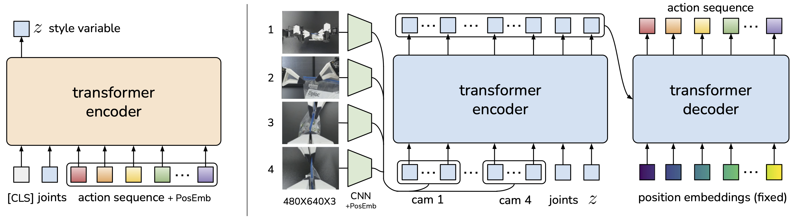
ACT is a Conditional VAE (CVAE) with two transformer-based halves:
- CVAE encoder (training only, left): a BERT-like transformer encoder takes a learned [CLS] token, the current joint positions, and the target action sequence from the demonstration. The output at
[CLS]predicts the mean and variance of the style variable (diagonal Gaussian). - CVAE decoder / policy (right): a transformer encoder–decoder takes 4 RGB images (processed by per-camera ResNet encoders with 2D sinusoidal position embeddings), the current joint positions, and , and predicts the next target joint positions for both arms.
At test time the CVAE encoder is discarded and is set to the mean of the prior (zero), making the policy deterministic.
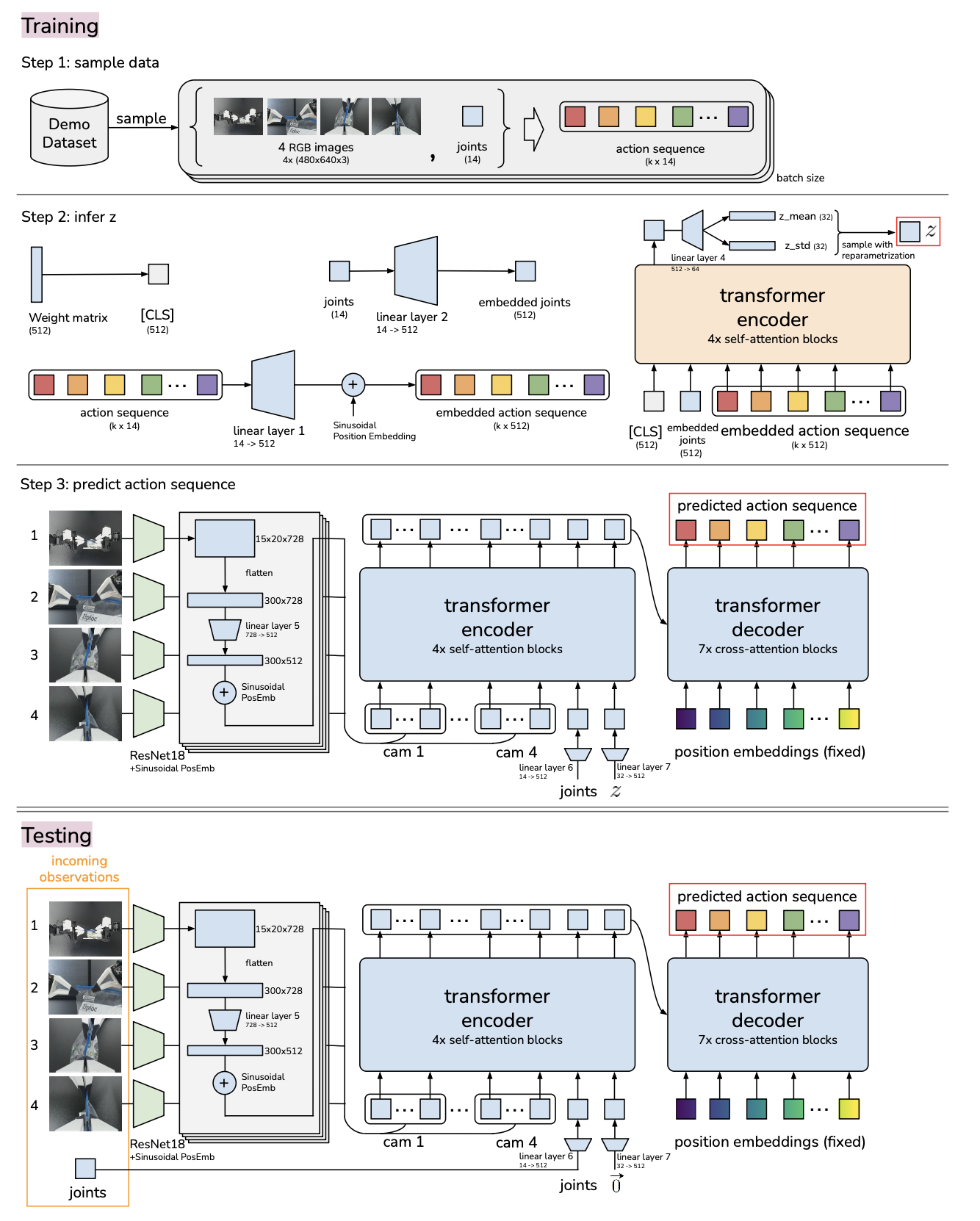
More detailed diagram:
What are the inputs and outputs of ACT at inference time?
Inputs:
- 4 RGB images at 480×640 from commodity webcams.
- Current joint positions of the two follower robots (7 + 7 = 14 DoF).
Output:
- A tensor of absolute target joint positions for the next timesteps (both arms).
Targets are then tracked by the low-level, high-frequency PID controllers inside the Dynamixel motors.
What is action chunking in ACT, and why does it help?
Instead of predicting a single action per step, the policy models
i.e. a sequence of future actions from one observation. Every steps the agent observes, generates actions, and executes them open-loop.
Why it helps: it reduces the effective horizon of the task by a factor of , which mitigates the compounding-error problem in behavioral cloning (small per-step errors drift the state off the training distribution). Empirically, success climbs from 1% at to 44% at before slightly tapering.
What is temporal ensembling in ACT, and how are overlapping chunks combined?
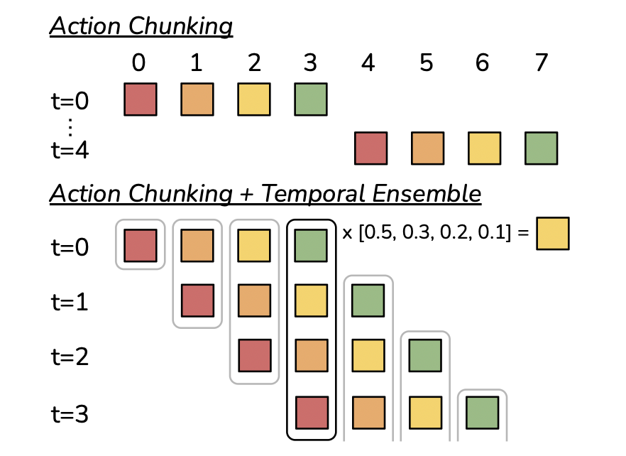
To avoid jerky switches between "observe" and "execute" phases, the policy is queried at every timestep, producing overlapping chunks that all propose an action for time .
These are combined with a weighted average:
where is the weight of the oldest proposed action and controls how fast newer predictions dominate. This smooths trajectories without slowing the control loop and requires no extra training.
Why is ACT trained as a CVAE rather than a plain regression to actions?
The problem — human demonstrations are multi-modal: for the same observation , a teleoperator may validly choose different action sequences on different takes (e.g. approach a cup from the left or from the right). A deterministic regressor trained with MSE/L1 on all these takes averages them and outputs the mean of the valid options, which often is not itself valid (averaging "go left" and "go right" → "go straight through the cup"). This is known as mode averaging / mode collapse.
What a CVAE is — a conditional variational autoencoder models as , where is a latent "style" variable drawn from a simple prior (unit Gaussian). Intuition: picks which mode you're in (e.g. "left-approach style") and the decoder produces the sequence consistent with that style. Because different takes get different 's, the decoder never has to blend them.
Training uses a standard VAE-style ELBO:
- an encoder infers which produced the observed demonstration,
- a decoder reconstructs the action sequence,
- loss = reconstruction (L1 on actions) + KL pulling toward the prior so stays well-behaved.
At test time the encoder is thrown away and is set to the prior mean (zero), giving one deterministic trajectory — you don't need to pick a style yourself.
Why it matters here — ablation: on scripted (deterministic) data, removing the CVAE objective barely changes performance because there's only one mode. On human data, success drops from 35.3% → 2%, showing the CVAE objective is essential whenever demonstrations contain genuine human variability.
How is the style variable used at train vs test time in ACT?
Training: the CVAE encoder sees the current joint positions and the target action sequence (but not the images, for speed) and outputs a diagonal-Gaussian . is sampled via the reparameterization trick and fed to the decoder. Loss = L1 reconstruction on actions + KL to a unit-Gaussian prior.
Test: the encoder is discarded. is set to the mean of the prior (zero vector), so given an observation the policy output is deterministic, which is useful for reproducible evaluation.
ACT makes several non-obvious design choices around actions and loss. What are they, and why?
- Leader joint positions as actions (not follower): the force applied is implicitly encoded in the difference between leader and follower joints via the low-level PID controller. Using follower joints would lose this information.
- Absolute target joint positions (not deltas): delta-action parameterization degrades performance.
- L1 reconstruction loss (not L2): L1 yields more precise modeling of the action sequence — important for fine manipulation.
- 50 Hz control rate: dropping to 5 Hz (typical of prior deep-imitation work) harms performance on precise tasks.
What are ACT's model size, training cost, and inference latency?
- ~80M parameters, trained from scratch per task.
- ~5 hours of training on a single 11 GB RTX 2080 Ti.
- ~0.01 s per forward pass at inference, which comfortably supports the 50 Hz control loop (especially combined with action chunking so a single forward pass yields actions).
- Data budget: 50 demos per task (100 for Thread Velcro) ≈ 10–20 min of demonstration data per task.