Diffusion Policy: Visuomotor Policy Learning via Action Diffusion
Draw and describe the Diffusion Policy architecture, and explain the observation (), prediction () and action () horizons.
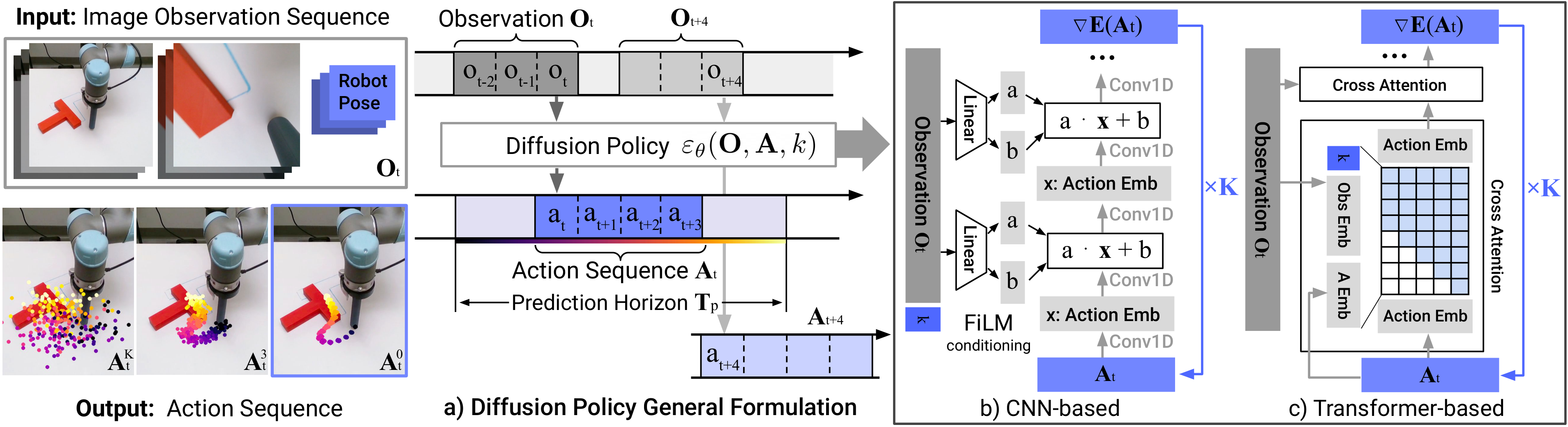
At environment time step the policy:
- Takes the last steps of observation, (images + robot pose).
- Starts from a pure-noise action sequence of length .
- Runs denoising iterations with noise-prediction network , producing , the predicted -step action sequence.
- Executes only the first steps of open-loop, then re-plans (receding-horizon control).
Notation convention: superscript indexes the diffusion iteration (since subscript is already taken by env time). Typical values: , , , training / inference via DDIM.
Write the conditional denoising update used at inference in Diffusion Policy and explain every symbol.
Starting from , this runs for to produce the clean action sequence .
- : action sequence of length at diffusion iteration (noisy for large , clean at ).
- : conditioning observation. It is only fed in, never denoised, so the vision encoder runs once per control step regardless of .
- : noise-prediction network; predicts the noise currently contaminating .
- : step size on the predicted noise (analogous to a learning rate; see gradient-descent card).
- : std of the Gaussian noise re-injected to keep the process stochastic (Langevin).
- : overall rescale, typically slightly to improve stability (Ho et al. 2020).
The triple is a function of and constitutes the noise schedule (DP uses the square-cosine schedule from iDDPM). It plays the role of learning-rate scheduling.
The standard DDPM update is the same equation with and folded into the schedule.
Give the training loss for Diffusion Policy, and explain how the noisy input is constructed.
Per training step:
- Sample from the demonstration dataset.
- Sample a diffusion iteration .
- Sample noise scaled by the schedule for step .
- Form the noisy action and let predict the noise that is added.
Why this works. This is exactly the DDPM -matching loss applied to action sequences conditioned on . The paper's compact notation is a shorthand: in the DDPM notation it would be written , where the variance of is set by the schedule at step . It has been shown that minimising this simple MSE also minimises the variational lower bound on , so we get proper density modelling with a plain regression loss.
Because is only conditioning (never noised), gradients flow through it and the vision encoder is trained end-to-end with .
Why can we interpret one step of the diffusion denoising update as noisy gradient descent on an energy landscape, and what does represent in this view?
Strip the bias/scale from the update:
Compare to gradient descent on some scalar energy :
So is effectively predicting the gradient field , and one denoising iteration is one step of (noisy) gradient descent toward a local minimum of .
Running such steps with added Gaussian noise is Stochastic Langevin Dynamics; it samples from rather than greedily descending to a single point. Noise lets trajectories hop between basins, which is exactly what lets the policy express multiple action modes instead of collapsing to the mean of the demonstrations.
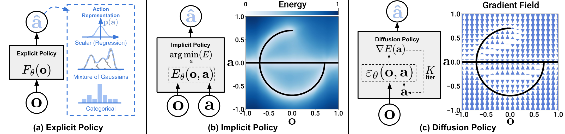
(c) Diffusion Policy denoises noise into actions by following a learned gradient field.
Why is Diffusion Policy more stable to train than an Implicit Behavioral Cloning (IBC)? Derive the key observation about the normalisation constant.
IBC represents the policy as an Energy-Based Model:
, the integral of over the whole action space, is intractable. IBC estimates it with an InfoNCE-style loss using negative action samples :
Poor negatives -> bad estimate -> training instability. Empirically IBC's train MSE and eval success both oscillate.
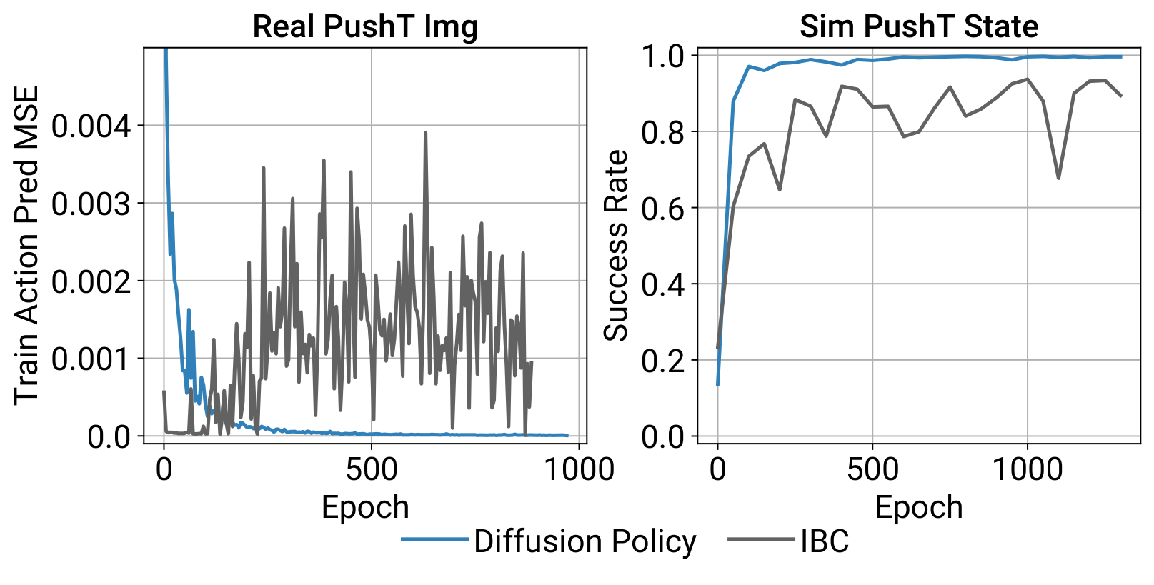
Diffusion Policy sidesteps entirely by modelling the score function instead of :
The term vanishes under , it's a constant w.r.t. . So neither training (MSE on noise) nor inference (Langevin steps) ever touches , and training is stable.
How does Diffusion Policy end up expressing multimodal action distributions, and where does the multimodality come from?
Multimodality arises from two stochastic sources in the Langevin sampler:
- Stochastic initialisation: each rollout starts from a fresh . Different initial points land in different convergence basins of the (implicit) energy .
- Injected Gaussian noise per iteration: the term in the update lets samples hop between basins during the denoising steps rather than deterministically rolling into the nearest one.
Because learns a gradient field over the whole action space (not a single-mode parametric distribution like a Gaussian or GMM), Stochastic Langevin Dynamics can, in principle, sample any normalisable . Combined with action-sequence prediction, this also gives temporal consistency: the whole -step chunk is sampled jointly from one mode, so consecutive actions don't alternate between "go left" and "go right".
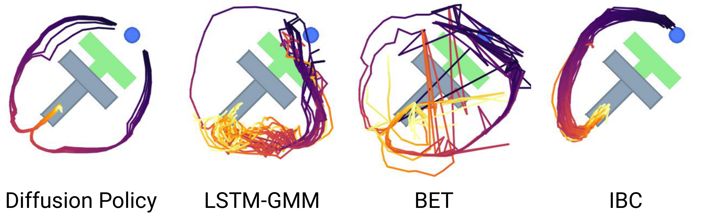
Pushing the T-block into the target: either left or right around it is valid. Diffusion Policy commits cleanly to one mode per rollout; LSTM-GMM/IBC are biased, BET jitters between modes.
Compare the CNN-based and Transformer-based Diffusion Policy backbones: how is the observation injected, and when would you use each?
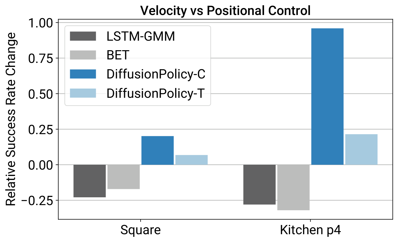
CNN-based (default): a 1-D temporal U-Net over the action sequence. and the diffusion step are injected via FiLM (Feature-wise Linear Modulation): per-channel affine applied at every conv layer. Works out-of-the-box on most tasks with little tuning. Weakness: temporal conv has a low-frequency inductive bias, so it over-smooths fast-changing actions (e.g. velocity control).
Transformer-based (time-series diffusion transformer): noisy actions are the input tokens of a minGPT-style decoder; a sinusoidal embedding of is prepended as the first token; an MLP-encoded is fed via cross-attention in each decoder block; causal self-attention within actions. Output tokens predict . Better on high-frequency / velocity-control tasks but more hyperparameter-sensitive.
Recommendation: start with CNN; switch to the transformer only if the task has rapid, sharp action changes.
What are the key design decisions that make Diffusion Policy practical on a real robot (action space, execution, inference speed)?
- Position control > velocity control. Surprising, because most BC baselines use velocity. Reasons: (i) position actions are more multimodal. Diffusion Policy handles this well, baselines (GMM, k-means) don't; (ii) position control suffers less from compounding error over long action chunks.
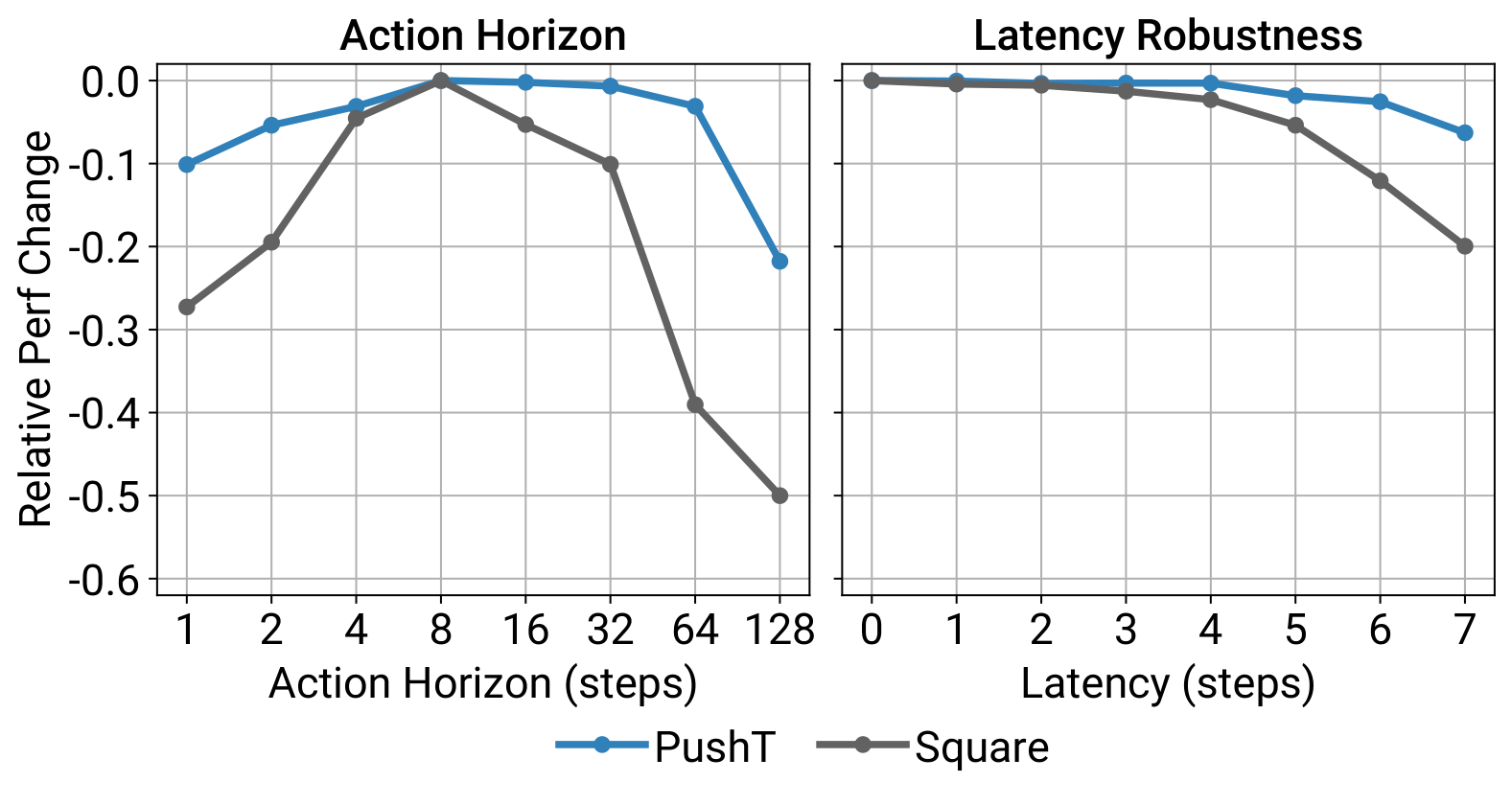
- Receding-horizon action chunking. Predict steps, execute only , then replan. Balances temporal consistency (large ) vs. reactivity (small ). Ablation shows an interior sweet spot around .
- Visual conditioning, not joint modelling. Model instead of (Diffuser-style). → the vision encoder runs once per control step regardless of denoising iterations; and it can be trained end-to-end with .
- End-to-end ResNet-18 with two tweaks: spatial-softmax pooling (preserves spatial info) and GroupNorm instead of BatchNorm (stable with EMA weights, which DDPMs use).
- DDIM for fast inference. DDIM decouples training and inference iteration counts. DP uses training, inference → ~0.1 s per forward pass on a 3080, enough for real-time closed-loop control.
- Action normalisation to . DDPMs clip predictions to each step, so zero-mean/unit-variance normalisation would make part of action space unreachable.
What is the control-theory sanity check for Diffusion Policy on a linear dynamical system with linear feedback demonstrations, and what does it reveal about the general case?
Take an LTI plant with LQR demonstrations:
Single-step prediction (). The MSE-optimal denoiser for has closed form
Plug into the DDIM update → Langevin converges to the unique global minimum . ✓
Multi-step prediction (). The optimal denoiser gives , i.e. to predict future actions the policy implicitly learns a (task-relevant) dynamics model by unrolling the closed-loop system.
Takeaway. Even in the simple LTI case, action-sequence prediction forces the network to encode dynamics; in the nonlinear case this becomes harder and inherently multimodal — which is exactly the regime where the diffusion formulation pays off.
LTI = Linear Time-Invariant. A dynamical system whose next state is a linear function of the current state and input, with matrices that do not change over time:
- (state transition) and (input matrix) are constant.
- is process noise.
LQR = Linear Quadratic Regulator. The optimal controller for an LTI system under a quadratic running cost
where penalises state error and penalises control effort. Minimising yields a linear state-feedback law
with gain obtained by solving the discrete-time Riccati equation.
Why the paper uses this setting. LTI + LQR is the classic "textbook" controllable case: known linear dynamics + quadratic cost → closed-form optimal linear policy. Because the ground-truth policy is simple and known, the optimal denoiser can be derived analytically, giving a clean sanity check that Diffusion Policy recovers the right controller in the limit.