π₀: A Vision-Language-Action Flow Model for General Robot Control
Describe the π₀ architecture: backbone, robotics-specific inputs/outputs, total parameter count, and how it differs from prior VLAs like RT-2 / OpenVLA.
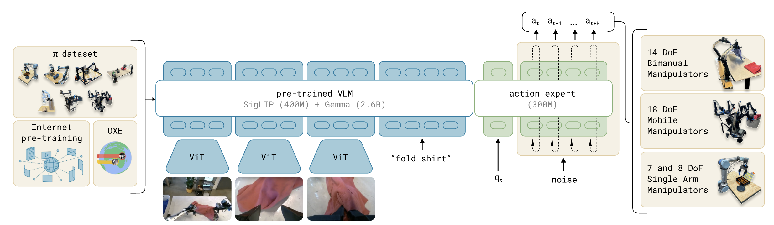
π₀ is a 3.3B-parameter VLA built on the PaliGemma 3B VLM (frozen recipe, then further trained), augmented with a 300M action expert for robot-specific tokens.
Inputs: , i.e. 2–3 RGB images, a language command, and the proprioceptive state (joint angles). Inputs follow the standard late-fusion VLM recipe: images go through a ViT, are linearly projected into the language embedding space, and concatenated with text tokens.
Output: an action chunk with , produced by conditional flow matching rather than autoregressive token prediction.
Key departure from RT-2 / OpenVLA: instead of discretizing actions into 256 bins and emitting them as text tokens with cross-entropy, π₀ emits continuous actions via a flow-matching head. This unlocks (i) full 50 Hz action chunks, (ii) high-frequency dexterous tasks (laundry folding, eggs into a carton), where autoregressive discretization breaks down.
π₀ is implemented as a mixture of experts with two experts, not a separate transformer. What are the two experts, what tokens go to each, and where do they interact?
π₀ is a single transformer with two parallel sets of weights ("experts"); each token is routed to exactly one expert and the experts only interact in the self-attention layers (Q/K/V mix between blocks).
| Expert | Tokens routed here | Init |
|---|---|---|
| VLM backbone (Gemma 2B, ~3B incl. ViT) | (images + language) | PaliGemma |
| Action expert (~300M) | (proprio state + noisy action chunk) | From scratch |
Why this design (vs. one shared transformer like Transfusion):
- The robotics tokens were not seen during VLM pre-training, so giving them their own weights avoids polluting the pre-trained features.
- Inference loops over flow-matching steps. The action expert is the part that runs , so making it smaller (
width=1024, mlp_dim=4096vs. backbone'swidth=2048, mlp_dim=16384) directly speeds up inference. Width and mlp-dim don't have to match between experts because they only meet in attention. - Empirically a separate weight set for action/state tokens improved performance over the shared-weights Transfusion variant.
Sketch the blockwise causal attention mask that π₀ uses. Why three blocks, and what does each block buy you at inference time?
Three blocks, with full bidirectional attention inside each and strict ordering between them:
Tokens in block can attend to blocks but not to later blocks.
Why split this way:
- Block 1 holds exactly the modalities seen in PaliGemma pre-training; preventing them from attending to the new (robotics) tokens minimises distribution shift from the VLM pre-training.
- Block 2 () is its own block because the proprioceptive state does not change across the 10 flow-matching integration steps at one control step. Isolating it lets its K/V be cached and reused across all 10 forward passes.
- Block 3 is the only block that changes per integration step. It uses full bidirectional self-attention internally so all action tokens see each other (this is the action expert), and it can attend to blocks 1 and 2 to read the observation/state.
Net effect: per control step the prefix forward pass runs once (32 ms), then only the action-token forward pass repeats 10 times (27 ms total) since blocks 1 and 2 are cached.
Write the conditional flow-matching training loss used by π₀, and explain what is being matched.
Subscripts are robot timesteps, superscripts are flow-matching timesteps.
Per training step:
- Sample a clean chunk and observation from the demonstration data.
- Sample noise and a flow timestep from a beta distribution.
- Form the noisy action chunk along the linear (optimal-transport) probability path:
- The network predicts the denoising vector field , i.e. the velocity that maps noise toward the data along the path.
Note: is pure noise and is clean data, the opposite of the DDPM convention. Action tokens use full bidirectional attention within block 3 so the network sees the whole chunk when predicting the velocity field.
Write the π₀ inference rule for generating an action chunk, list the integration parameters, and explain the KV-cache trick that makes it fast.
Start from and integrate the learned vector field from to with forward Euler:
Defaults: , so 10 integration steps.
KV-cache trick. The observation does not change across the 10 integration steps, and the attention mask prevents prefix tokens from attending to action tokens. So:
- Run the prefix forward pass once to populate the K/V cache for blocks 1 and 2 (images + language + state).
- For each of the 10 integration steps, only re-run the suffix corresponding to the noisy action tokens; they read the cached prefix K/V via cross-block attention.
Measured cost on an RTX 4090 with 3 cameras: image encoders 14 ms + observation forward 32 ms + 10× action forward 27 ms = 73 ms total on-board (86 ms off-board with WiFi). Because actions are produced at once, this comfortably supports 50 Hz control: the 50 Hz robots replan every 25 actions = 0.5 s, the 20 Hz robots every 16 actions = 0.8 s.
Action chunks are executed open-loop; the authors tried temporal ensembling (averaging chunks from successive inferences) and found it hurt performance.
How is each noisy action in the chunk turned into a transformer embedding, and how is the flow-matching timestep injected?
Each noisy action vector is mapped to the action expert's embedding dimension by a 3-layer MLP that fuses the action with a sinusoidal embedding of :
where is a sinusoidal positional encoding of , , , , is the action dimension and the action expert's width (1024).
Same idea as DiT's adaLN-Zero: condition every action token on so the same shared weights can play different roles at different noise levels. Crucially, is fused per-token before the transformer, not via a separate global modulation, which keeps the architecture pure self-attention.
The transformer outputs at the action positions are then linearly projected back to the action dimension to produce the predicted velocity .
π₀ samples the flow-matching timestep from a shifted beta distribution instead of the uniform/logit-normal used for image generation. Why?
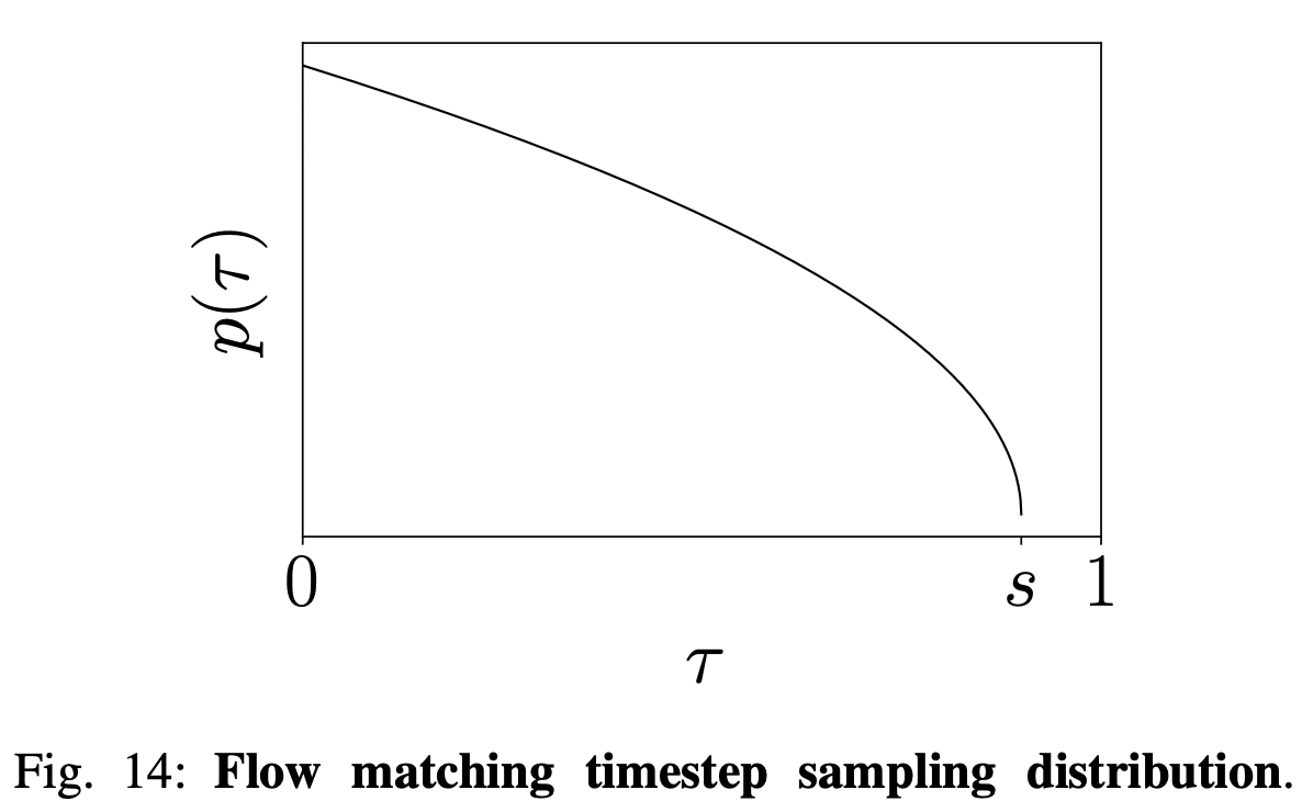
Distribution: , with cutoff . It (i) emphasises low (high noise) and (ii) never samples .
Why low ? Esser et al. (Stable Diffusion 3) sample logit-normal in the middle, arguing that:
- At high (low noise) the network just has to learn the identity.
- At low (high noise) the network just has to predict the mean of the data distribution.
π₀ argues the second claim does not hold for action prediction: the observation is highly informative and should sharply constrain the conditional action distribution . So learning at low is a hard problem, and you want to spend more samples there. (For images, the text label only weakly constrains the image, so learning the mean image is easy.)
Why a cutoff ? With Euler step size , you only need to learn at -values that the integrator will actually visit, namely . Points beyond are wasted. supports up to integration steps, far more than the 10 used.
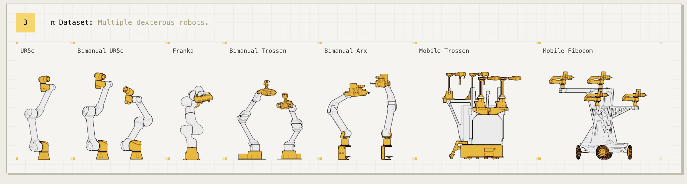
π₀ is trained jointly on 7 robot configurations with different DoF, gripper counts, and bases. How does it cope with the heterogeneous action/state spaces?
The configuration vector and action vector are always the same dimensionality, set to the largest robot in the dataset = 18 (two 6-DoF arms + 2 grippers + mobile base + vertical torso = 18 action dims).
Smaller robots are zero-padded: unused dimensions of and are filled with zeros. Robots with fewer than 3 cameras have the missing image slots masked out in attention.
Sample weighting addresses dataset imbalance (laundry folding has way more steps than UR5e tasks): each task–robot combination is weighted by where is its sample count. This down-weights over-represented combinations without ignoring them, similar in spirit to OXE's "Magic Soup" weighting and Octo's mixture weights.
The 7 platforms: UR5e (1×7-DoF), Bimanual UR5e (2×7-DoF), Franka (1×8-DoF), Bimanual Trossen (2×6-DoF, ALOHA-style), Bimanual ARX/AgileX (2×6-DoF), Mobile Trossen/ARX (2×6-DoF + nonholonomic base, 16-DoF action), Mobile Fibocom (2×6-DoF + holonomic base, 17-DoF action). Plus open-source data: OXE Magic Soup subset, Bridge v2, DROID — together ~9.1% of the mixture, with the in-house 903M timesteps making up the rest.
What is π₀'s pre-training / post-training recipe, and why is it intentionally two stages with different data quality?
Mirrors the LLM recipe (broad pre-training, narrow alignment), but applied to robot demonstrations.
| Stage | Data | Objective |
|---|---|---|
| Pre-training | Maximise diversity. All 903M in-house steps + OXE/Bridge/DROID; 7 robots, 68 tasks, including messy/sub-optimal trajectories and recovery behaviours; language labels include 2-second segment annotations, not just the overall task name. | Train a base model with broad capability and language grounding; not specialised. |
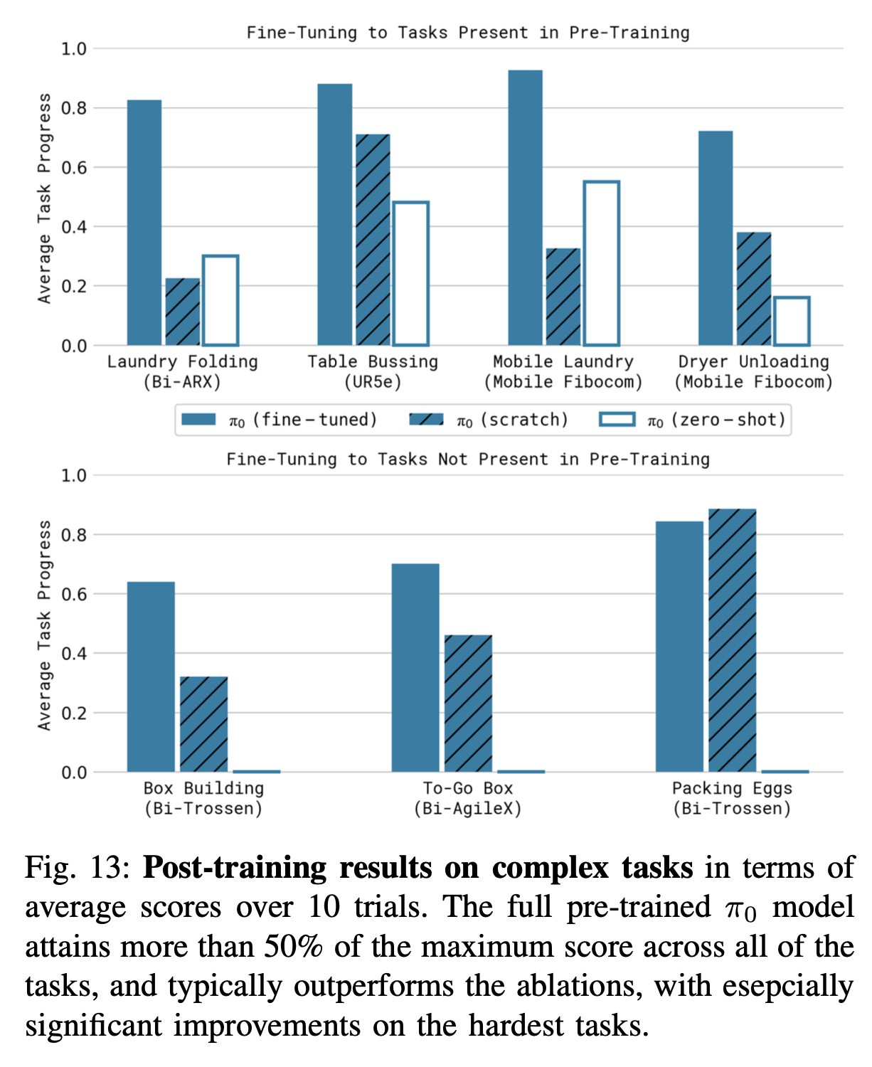
| Post-training | Maximise quality. Small (5–100 hr) curated, fluent, consistent strategy demos for one downstream task. | Specialise the base into a dexterous executor for that task. |
Why both:
- Pre-training only → fluent in coverage, but does not always exhibit the smooth, fluent strategy needed for hard tasks like laundry folding.
- Post-training only on clean data → no exposure to mistakes/recoveries, so the policy is brittle and cannot recover when something goes off-script.
- Combined → the model knows the fluent target behaviour from post-training data and inherits a repertoire of recoveries from pre-training data.
Empirically (Fig. 13) the gap pre-train+ft vs. ft-from-scratch is largest on the hardest tasks (laundry, box building), exactly where recovery matters most.
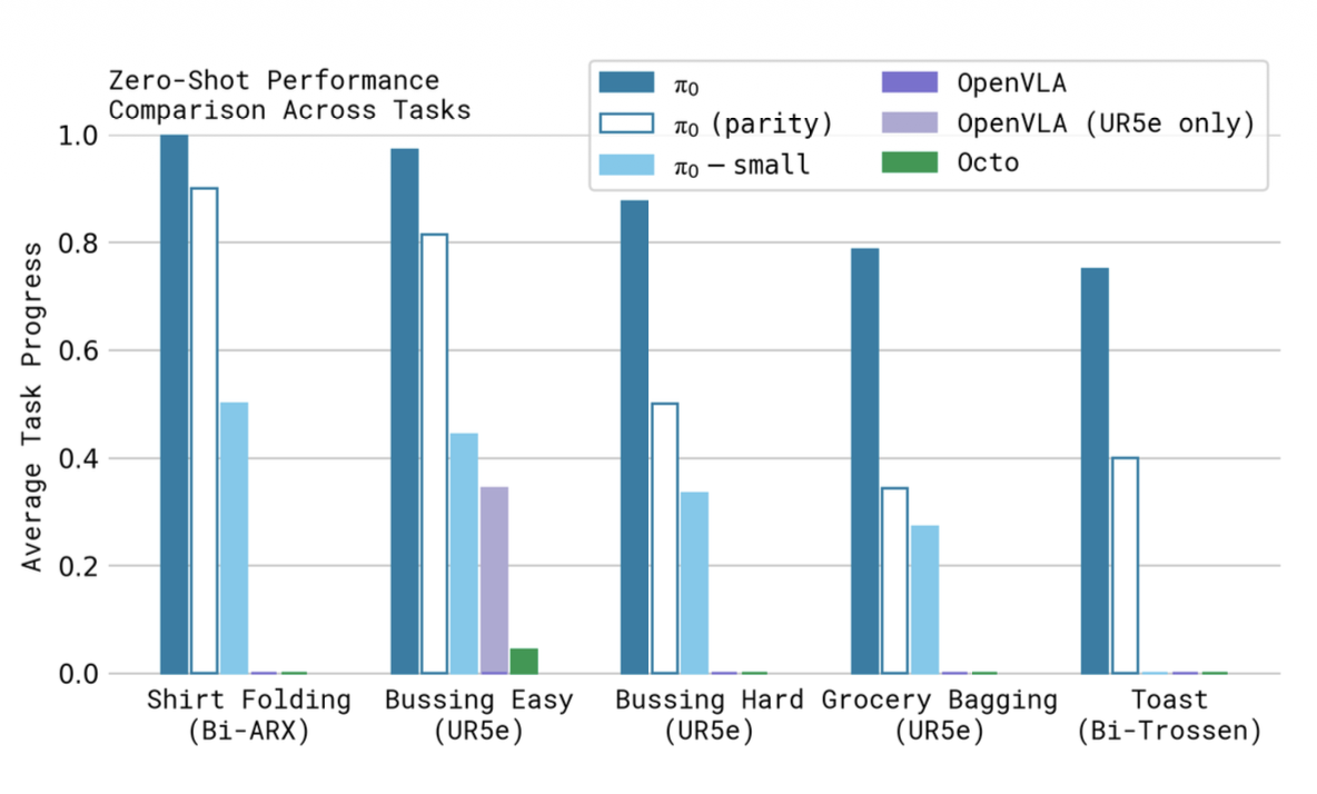
Why does π₀ choose flow matching with action chunking over autoregressive action tokenisation (RT-2, OpenVLA)?
Three concrete reasons, all about high-frequency dexterous control:
- Frequency. RT-2/OpenVLA emit one action per autoregressive call; with actions per chunk and 7+ dims each, autoregressive decoding is far too slow for 50 Hz control. π₀'s flow matching emits the whole 50-step chunk in 10 forward passes of the action expert (one for each integration step), independent of .
- Continuous, multimodal action distributions. Discretising into 256 bins per dim loses precision and forces a categorical model on what is fundamentally a continuous, often multimodal distribution (two valid grasp poses, two valid fold orders). Flow matching directly models as a continuous distribution via a learned vector field, the same advantage Diffusion Policy has over BC-MSE.
- No 256-token-vocab hack. OpenVLA had to overwrite the 256 least-used Llama vocab entries to make room for action tokens. π₀'s action expert is a separate, continuous head, so the VLM vocabulary stays untouched.
Empirically (Fig. 7), OpenVLA trained on the same mixture fails on the dexterous tasks, which the authors attribute primarily to the lack of action chunking and the autoregressive bottleneck.