Auto-Encoding Variational Bayes

What is the formula for variational lower bound, or evidence lower bound (ELBO) in variational Bayesian methods?


The evidence lower bound (ELBO) is defined as logpθ(x)DKL(qϕ(zx)pθ(zx))=Ezqϕ(zx)logpθ(xz)DKL(qϕ(zx)pθ(z))\log p_\theta(\mathbf{x}) - D_\text{KL}( q_\phi(\mathbf{z}\vert\mathbf{x}) \| p_\theta(\mathbf{z}\vert\mathbf{x}) ) = \mathbb{E}_{\mathbf{z}\sim q_\phi(\mathbf{z}\vert\mathbf{x})}\log p_\theta(\mathbf{x}\vert\mathbf{z}) - D_\text{KL}(q_\phi(\mathbf{z}\vert\mathbf{x}) \| p_\theta(\mathbf{z})) The lower bound part in the name comes from the fact that the KL divergence is always non-negative and thus ELBO is the lower bound of logpθ(x)\log p_\theta (\mathbf{x}).

Derive the ELBO loss function used for variational inference.


The goal in variational inference is to minimize DKL(qϕ(zx)pθ(zx))D_\text{KL}( q_\phi(\mathbf{z}\vert\mathbf{x}) | p_\theta(\mathbf{z}\vert\mathbf{x}) ) with respect to ϕ\phi.

Starting from the definition and expanding step-by-step: DKL(qϕ(zx)pθ(zx))=qϕ(zx)logqϕ(zx)pθ(zx)dzD_\text{KL}( q_\phi(\mathbf{z}\vert\mathbf{x}) \| p_\theta(\mathbf{z}\vert\mathbf{x}) ) = \int q_\phi(\mathbf{z} \vert \mathbf{x}) \log\frac{q_\phi(\mathbf{z} \vert \mathbf{x})}{p_\theta(\mathbf{z} \vert \mathbf{x})} d\mathbf{z}

Using p(zx)=p(z,x)/p(x)p(z \vert x) = p(z, x) / p(x): =qϕ(zx)logqϕ(zx)pθ(x)pθ(z,x)dz= \int q_\phi(\mathbf{z} \vert \mathbf{x}) \log\frac{q_\phi(\mathbf{z} \vert \mathbf{x})p_\theta(\mathbf{x})}{p_\theta(\mathbf{z}, \mathbf{x})} d\mathbf{z}

Expanding the logarithm: =logpθ(x)+qϕ(zx)logqϕ(zx)pθ(z,x)dz= \log p_\theta(\mathbf{x}) + \int q_\phi(\mathbf{z} \vert \mathbf{x})\log\frac{q_\phi(\mathbf{z} \vert \mathbf{x})}{p_\theta(\mathbf{z}, \mathbf{x})} d\mathbf{z}

Using p(z,x)=p(xz)p(z)p(z, x) = p(x \vert z) p(z): =logpθ(x)+Ezqϕ(zx)[logqϕ(zx)pθ(z)logpθ(xz)]= \log p_\theta(\mathbf{x}) + \mathbb{E}_{\mathbf{z}\sim q_\phi(\mathbf{z} \vert \mathbf{x})}\left[\log \frac{q_\phi(\mathbf{z} \vert \mathbf{x})}{p_\theta(\mathbf{z})} - \log p_\theta(\mathbf{x} \vert \mathbf{z})\right]

Therefore: DKL(qϕ(zx)pθ(zx))=logpθ(x)+DKL(qϕ(zx)pθ(z))Ezqϕ(zx)logpθ(xz)D_\text{KL}( q_\phi(\mathbf{z}\vert\mathbf{x}) \| p_\theta(\mathbf{z}\vert\mathbf{x}) ) = \log p_\theta(\mathbf{x}) + D_\text{KL}(q_\phi(\mathbf{z}\vert\mathbf{x}) \| p_\theta(\mathbf{z})) - \mathbb{E}_{\mathbf{z}\sim q_\phi(\mathbf{z}\vert\mathbf{x})}\log p_\theta(\mathbf{x}\vert\mathbf{z})

Once rearrange the left and right hand side of the equation,

logpθ(x)DKL(qϕ(zx)pθ(zx))=Ezqϕ(zx)logpθ(xz)DKL(qϕ(zx)pθ(z))\log p_\theta(\mathbf{x}) - D_\text{KL}( q_\phi(\mathbf{z}\vert\mathbf{x}) \| p_\theta(\mathbf{z}\vert\mathbf{x}) ) = \mathbb{E}_{\mathbf{z}\sim q_\phi(\mathbf{z}\vert\mathbf{x})}\log p_\theta(\mathbf{x}\vert\mathbf{z}) - D_\text{KL}(q_\phi(\mathbf{z}\vert\mathbf{x}) \| p_\theta(\mathbf{z}))

The left side of the equation is exactly what we want to maximize when learning the true distributions: we want to maximize the (log-)likelihood of generating real data (that is logpθ(x)\log p_\theta(\mathbf{x})) and also minimize the difference between the real and estimated posterior distributions (the term DKLD_\text{KL} works like a regularizer). Note that pθ(x)p_\theta(\mathbf{x}) is fixed with respect to qϕq_\phi.

The negation of the above defines our loss function:

LVAE(θ,ϕ)=logpθ(x)+DKL(qϕ(zx)pθ(zx))L_\text{VAE}(\theta, \phi) = -\log p_\theta(\mathbf{x}) + D_\text{KL}( q_\phi(\mathbf{z}\vert\mathbf{x}) \| p_\theta(\mathbf{z}\vert\mathbf{x}) )

Which can also be written as: LVAE(θ,ϕ)=Ezqϕ(zx)logpθ(xz)+DKL(qϕ(zx)pθ(z))L_\text{VAE}(\theta, \phi) = - \mathbb{E}_{\mathbf{z} \sim q_\phi(\mathbf{z}\vert\mathbf{x})} \log p_\theta(\mathbf{x}\vert\mathbf{z}) + D_\text{KL}( q_\phi(\mathbf{z}\vert\mathbf{x}) \| p_\theta(\mathbf{z}) )

Optimal parameters are found by: θ,ϕ=argminθ,ϕLVAE\theta^{*}, \phi^{*} = \arg\min_{\theta, \phi} L_\text{VAE}

VAE-graphical-model.png 
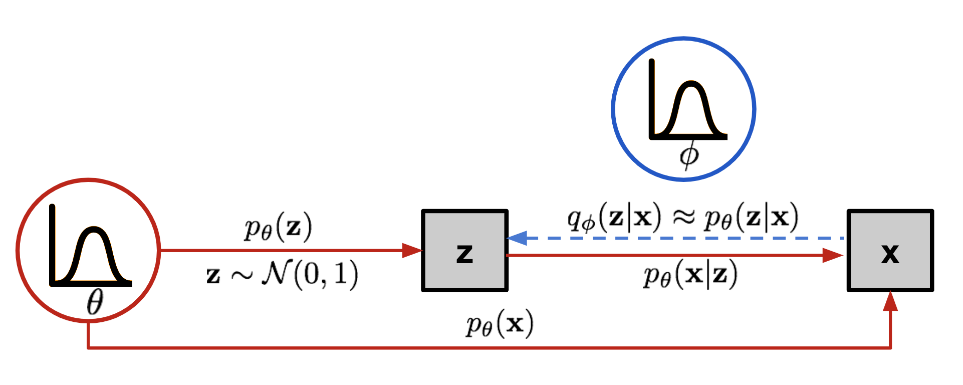
The graphical model involved in Variational Autoencoder. Solid lines denote the generative distribution pθ(.)p_\theta(.) and dashed lines denote the distribution qϕ(zx)q_\phi(z \mid x) to approximate the intractable posterior pθ(zx)p_\theta(z \mid x). Source: https://lilianweng.github.io/posts/2018-08-12-vae/

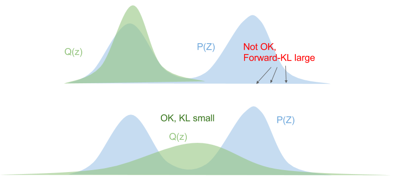
Why does ELBO use the reverse Kullback-Leibler divergence DKL(qϕpθ)D_\text{KL}(q_\phi | p_\theta) instead of the forward KL divergence DKL(pθqϕ)D_\text{KL}(p_\theta | q_\phi)?


KL divergence is not a symmetric distance function, i.e. DKL(qϕpθ)DKL(pθqϕ)D_\text{KL}(q_\phi | p_\theta) \ne D_\text{KL}(p_\theta | q_\phi). Let's consider the forward KL divergence: DKL(pq)=zp(z)logp(z)q(z)=Ep(z)[logp(z)q(z)]D_\text{KL}(p | q) = \sum_z p(z) \log \frac{p(z)}{q(z)} = \mathbb{E}_{p(z)}{\big[\log \frac{p(z)}{q(z)}\big]} This means that we need to ensure that q(z)>0q(z) > 0 wherever p(z)>0p(z) > 0. The optimized variational distribution Q(Z)Q(Z) is known as zero-avoiding. forward-KL.png 
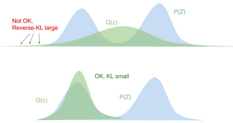
The reversed KL divergence has the opposite behaviour. DKL(qp)=zq(z)logq(z)p(z)=Eq(z)[logq(z)p(z)]D_\text{KL}(q | p) = \sum_z q(z) \log \frac{q(z)}{p(z)} = \mathbb{E}_{q(z)}{\big[\log \frac{q(z)}{p(z)}\big]} If p(z)=0p(z) = 0, we must ensure that q(z)=0q(z) = 0, othewise the KL divergence blows up. This is known as zero-forcing. reverse-KL.png

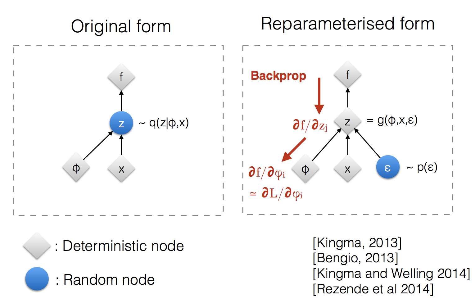
What is the reparameterization trick used in variational autoencoders?


Variational autoencoders sample from zqϕ(zx)\mathbf{z} \sim q_\phi(\mathbf{z}\vert\mathbf{x}). Sampling is a stochastic process and therefore we cannot backpropagate through it. To make it differentiable, the reparameterization trick is introduced. It is often possible to express the random variable z\mathbf{z} as a deterministic variable z=Tϕ(x,ϵ)\mathbf{z} = \mathcal{T}_\phi(\mathbf{x}, \boldsymbol{\epsilon}), where ϵ\epsilon is an auxiliary independent random variable and the transformation function Tϕ\mathcal{T}_\phi converts ϵ\boldsymbol{\epsilon} to z\mathbf{z}.

For example, a common choice of the form of qϕ(zx)q_\phi(\mathbf{z}\vert\mathbf{x}) is a multivariate Gaussian with a diagonal covariance structure: zqϕ(zx(i))=N(z;μ(i),σ2(i)I)\mathbf{z} \sim q_\phi(\mathbf{z}\vert\mathbf{x}^{(i)}) = \mathcal{N}(\mathbf{z}; \boldsymbol{\mu}^{(i)}, \boldsymbol{\sigma}^{2(i)}\boldsymbol{I}) Using the reparameterization trick: z=μ+σϵ, where ϵN(0,I)\mathbf{z} = \boldsymbol{\mu} + \boldsymbol{\sigma} \odot \boldsymbol{\epsilon} \text{, where } \boldsymbol{\epsilon} \sim \mathcal{N}(0, \boldsymbol{I}) reparameterization-trick.png

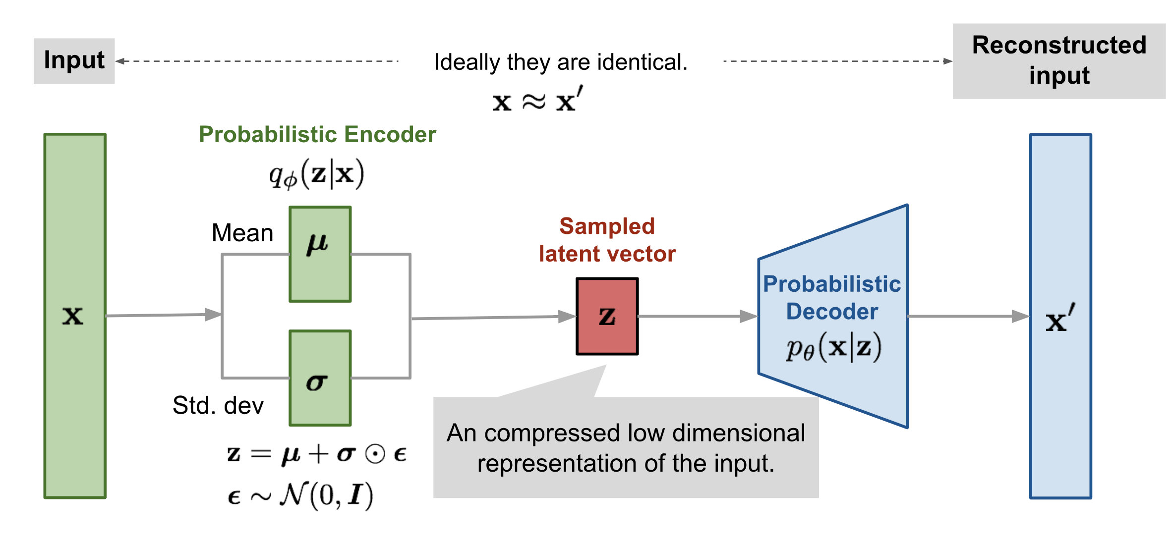
Draw the architecture of a variational autoencoder (VAE).

Machine Learning Research Flashcards is a collection of flashcards associated with scientific research papers in the field of machine learning. Best used with Anki or Obsidian. Edit MLRF on GitHub.